Scatterplots

In experiments, it often happens that two variables are measured in order to find out how they are related. For example, we suspect that there is a connection between a lot of sleep and higher school grades. To test this suspicion, we could now ask students over a period of time about their grades ( $x$ ), and also how much they slept the night before the exam ( $y$ ).

These data can then be plotted as points in a coordinate system (so-called scatterplots or correlation diagrams). Often a function is searched for, which describes these points as good as possible. So we want to fit a function to the data.

This is to be done "by hand". But of course there are also computer programs, which do this automatically ... .

Example 1

In the following, function equations are to be found which go as well as possible through the point sets below.

The link to the point sets is here. Attention, pressing the same button several times changes the point set a little bit, but not the function to be found.

Procedure:

consider the type of function (power function, linear function, exponential function)
consider from the points what the possible parameters could be (for example, does it have a vertex, where? How big is $A$ , etc.).

To check how well the function equation fits, you can enter it in the input field below the scatterplot. Write for example

f(x)=2*(x+1)^2-5

To try other function equations, simply re-enter the $f$ . The $f$ can also be deleted with the command

delete(f)

Below we discuss how to determine the power $p$ when fitting a power function from the data points. Until now, we have always had to hope that the power is of the form $p=n, p=-n$ , or $p=1/n$ . But what if another power would fit the data better, such as $p=2.324$ ? We discuss this using a concrete example:

Example 2

In an experiment, a rubber ball is dropped from a height of 1.8m. The speed of the ball is measured as a function of the distance the ball has already travelled when it falls. The data are summarized in a table:

\begin{array}{c|c} \text{$x$=Distance (m)} & \text{$y$=Velocity (m/s)} \\ \hline 0.00 & 0.00\\ 0.04 & 0.82\\ 0.16 & 1.71\\ 0.35 & 2.45\\ 0.59 & 3.05\\ 0.89 & 3.74\\ 1.26 & 4.45\\ \end{array}

Plot this data on a scatterplot and fit a power function to the data. Then make a prediction of how fast the ball will hit the ground.

Click right to see the calculation.

Show

Calculating $f$

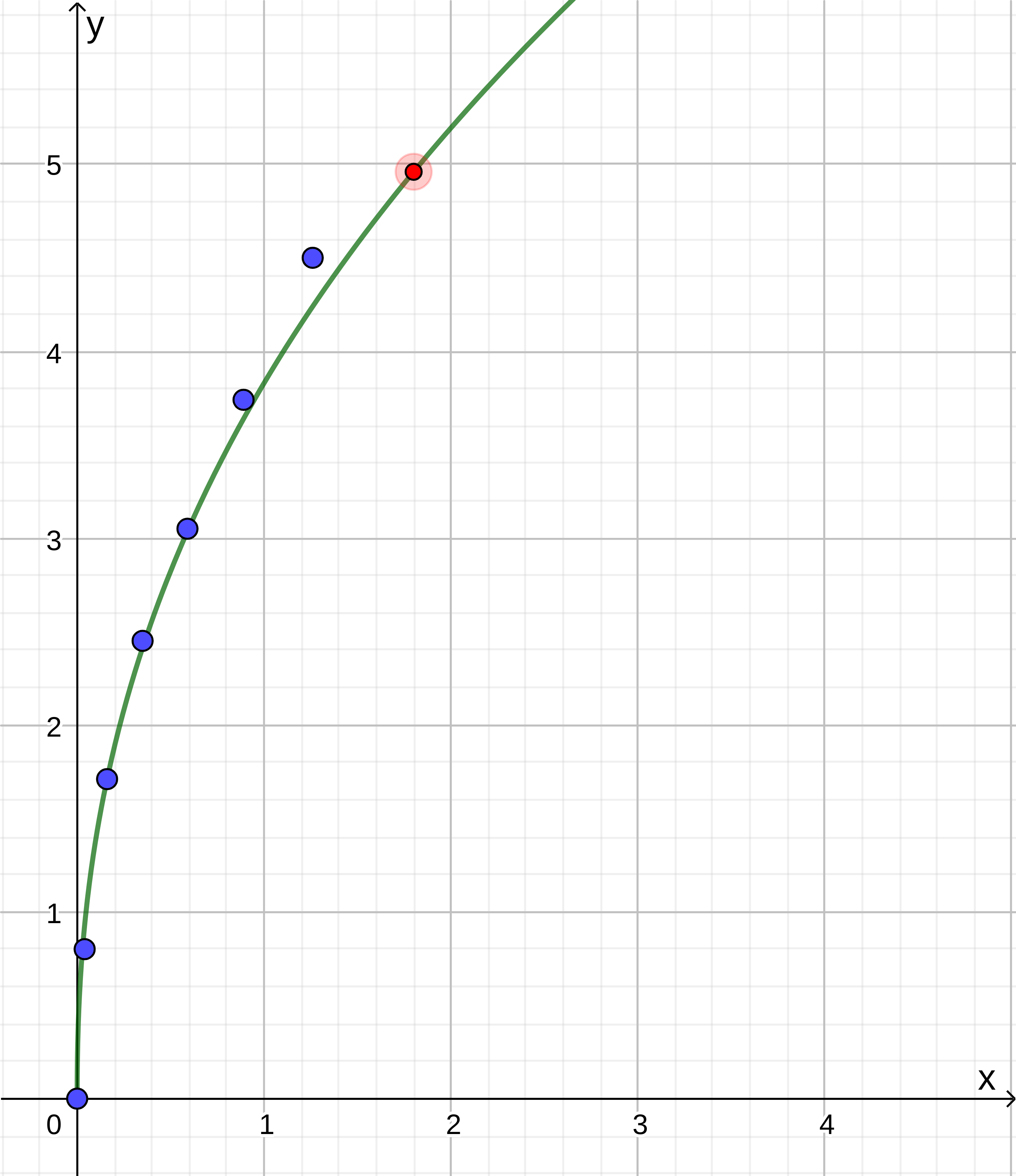
The scatterplot is shown below.

$S$ is the coordinate origin, so it is

f(x)=Ax^{p}

To find $A$ and $p$ , we put in two points. We already needed the zero point, so we need two other points, like $A(0.16\vert 1.71$ and $B(0.59\vert 3.74)$ . We then have

f(0.16)=1.71 \rightarrow A\cdot 0.16^p = 1.71

f(0.59)=3.74 \rightarrow A\cdot 0.59^p = 3.05

So we have two equations (and two unknowns). From the first equation follows

A=\frac{1.71}{0.16^p}

If we substitute the expression for $A$ into the second equation, we get

\frac{1.71}{0.16^p} \cdot 0.59^p = 3.05

1.71 \cdot \frac{0.59^p}{0.16^p} =3.05

1.71 \cdot \left(\frac{0.59}{0.16}\right)^p =3.05

\left(\frac{0.59}{0.16}\right)^p =\frac{3.05}{1.71}=1.78

We now take the logarithm to base $10$ on both sides, and get

\log_{10}\left( \left(\frac{0.59}{0.16}\right)^p\right) = \log_{10}(1.78)

p\cdot \underbrace{\log_{10}\left( \frac{0.59}{0.16}\right)}_{0.567} = \underbrace{\log_{10}(1.78)}_{0.25}

For repetition, in the last step we have used the logarithm rule

\log_{10}(a^p)=p\cdot \log_{10}(a)

Thus

p=\frac{0.25}{0.567}=0.44

To find $A$ , we put $p$ in one of the two equations. We take the first one, i.e.

A\cdot 0.16^p = 1.71

A\cdot \underbrace{0.16^{0.44}}_{0.45} = 1.71

A=\frac{1.71}{0.45}=3.83

Thus we have the function

f(x)=\underline{3.83\cdot x^{0.44}}

As the longer calculation shows, the fitted function is given by

f(x)=\underline{3.83\cdot x^{0.44}}

Indeed, the fit is not bad, as the diagram below points out. We can now also make a prediction about the impact velocity:

y_{impact} = f(1.8)=3.83\cdot 1.8^{0.44} = \underline{4.96 m/s}

This is the red dot in the scatterplot. It should be noted here that only two data points were used to calculate $f$ , and depending on the choice of these points from the table above, slightly different function $f$ will result. Ideally, one would use all data points. Such methods do indeed exist, and are routinely used (such as regression).

Exercise 1

The graph of a reference function $x^p$ is shifted $2$ to the right, and then passes through the points $A(3\vert 3.2)$ and $B(5.9\vert 21.51)$ . Determine the function equation of the shifted function $f$ .

Solution

It is

f(x)=A(x-2)^p

and

f(3)=3.2 \rightarrow A\cdot 1^p=3.2

f(5.9)=21.51 \rightarrow A\cdot 3.9^p=21.51

Because of $1^p=1$ follows

A=3.2

Insert into the second equation

3.2\cdot 3.9^p=21.51

3.9^p=\frac{21.51}{3.2}=6.722

Apply the logarithm on both sides:

\log_{10}(3.9^p)=\log_{10}(6.722)

thus

p\cdot \log_{10}(3.9)=\log_{10}(6.722)

and

p=\frac{\log_{10}(6.722)}{\log_{10}(3.9)}=1.4

We get the function

f(x)=\underline{3.2\cdot (x-2)^{1.4}}

Scatterplots

Calculating ff

Calculating $f$