Integral calculus

We have seen that differential calculus contributes useful concepts to

• geometry: $f'(x)$ is the slope of the tangent (section 04)
• dynamical systems: $f'(x)$ is the amplification factor of disturbances (section 21)
• measure of change: $f'(x)$ is the instantaneous speed (section 23)

And this is just the tip of the ice-berg. Important contributions to our understanding of nature, such as Albert Einstein's general relativity with its curved space-time geometry,

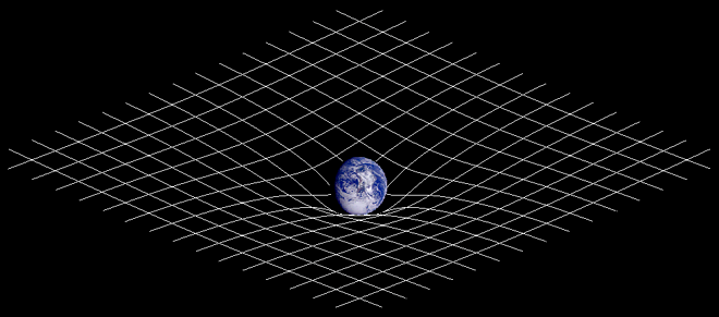
or Maxwell's equations describing how electromagnetic waves propagate in space (e.g light),

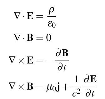
to name just a few, all make heavy use of differential calculus. The curvature in general relativity, for example, describes how the surface changes, which can be expressed with differential calculus. And all the triangles $\nabla$ and $\frac{\partial}{\partial t}$ you see in Maxwell's equations are derivatives which describe how the Electromagnetic fields $E$ and $B$ change in time and space.

The next couple of sections is about integral calculus. While differential calculus is about how things change, integral calculus is about summing up or integrating the changes to form the whole. Thus, integral calculus can be seen as the inverse operation of differential calculus, in the sense that it undoes the effect of taking the derivative.

To illustrate the inverse operation business a little bit deeper, consider a ball falling from a tower of height $125m$ (uncollapse to see the animation).

Show

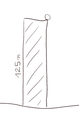
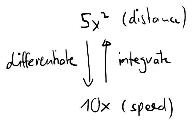
The distance that the ball has travelled after $x$ seconds (measured from the top of the tower) is

Or in physics terminology (with $g=9.81\approx 10$, I hope you remember ...), $s(t)=\frac{1}{2}g t^2$. The instantaneous speed is therefore

or again in physics talk $v(t)=s'(t)=gt$. So the speed increases, and the ball falls quicker and quicker. Let's plot the instantaneous speeds of the ball every $\Delta x =0.5 s$ in a table, together with the distance travelled by the ball.

So the ball has travelled $125m$ and therefore hitting the ground after $5s$ with an instantaneous speed of $50m/s$ (ignoring, of course, air friction). So with differential calculus we go from the distance travelled to instantaneous speed. With integral calculus we can go the other direction, from the instantaneous speed to the distance function:

How? Recall the approximation (see nudging the input, section 20)

where we use now $\Delta x$ rather than $h$. The smaller the value $\Delta x$ is, the better the approximation, but for now let's stick to the value

which is the same value we used above to create the table. The goal is to find the function $f(x)$, so this function is unknown in the approximation above. With the relation above we can start "rebuilding" the function $f$ just with the our knowledge that the derivative of $f$ is $f'(x)=10x$, step by step.

To do so, let's start with the time $x=0$. The problem dictates that at this point of time the distance travelled by the ball is $0$, as it is just about to start falling from the tower. So we have

Now let's try to figure out the value for $f(0.5)$. Using the approximation above with $x=0$, we get

So, we have an estimate of $f(0.5)$. But we can continue, using this value for the next step, to find $f(1)$:

Let's do another step and find $f(1.5)$:

I hope it is clear how we can go on reconstructing $f$. Let's see how well this works by adding these and all other values to the table from above:

As you can see, the estimates are reasonable, but not overwhelmingly good. But do not forget that we are working here only with approximations, and the approximations are better for smaller time interval length $\Delta x$. Uncollapse to play with $\Delta x$. You will see that for small values the reconstructed function is very close to the original function $f$.

Observe that to estimate $f$ we had to keep adding terms of the form

where $x=0.5, 1, 1.5, ...$ and $\Delta x = 0.5$. This process of adding these terms is, in essence, called integration. There are some details we still have to discuss, but the main message you should take away at the moment is that we can estimate the output of $f$ using its derivative $f'$ alone, and we do this by a process that involves adding many terms of the form $f'(x)\Delta x$.

In fact many experiments and theories start with measurements or hypothesis about the derivative of a function, $f'(x)$, although ultimately one wants to know $f$. Integral calculus is the tool that is applied to find then this $f$.

Differential calculus started with a small question: how can we determine the slope of a tangent to a curve? Integral calculus starts with a similar small question: how can we determine the area under a curve? This is the topic of the next sections.