Probability calculations with the normal distribution
Consider a random variable with mean and standard deviation which is normally distributed. Thus, the probability density function of is . Recall that the probability for to have a value in a given interval is the area under the probability density function
For example, if the mean is and the standard deviation is , the probability for to be between and is
Now, to actually calculate the probability, we have to find an antiderivative of the function
and with the fundamental theorem of calculus we then have
Unfortunately, the antiderivative cannot be expressed using any combination of the elementary functions like and so on. So we have to find the integral numerically using the calculator. (When calculators were still rare, people used large tables which listed the area under the curve for many different intervals.)
Use the calculator to determine the probability numerically by using the integral key on your calculator.
Hint: Later we will see that we can use the calculator's normcdf.
Solution
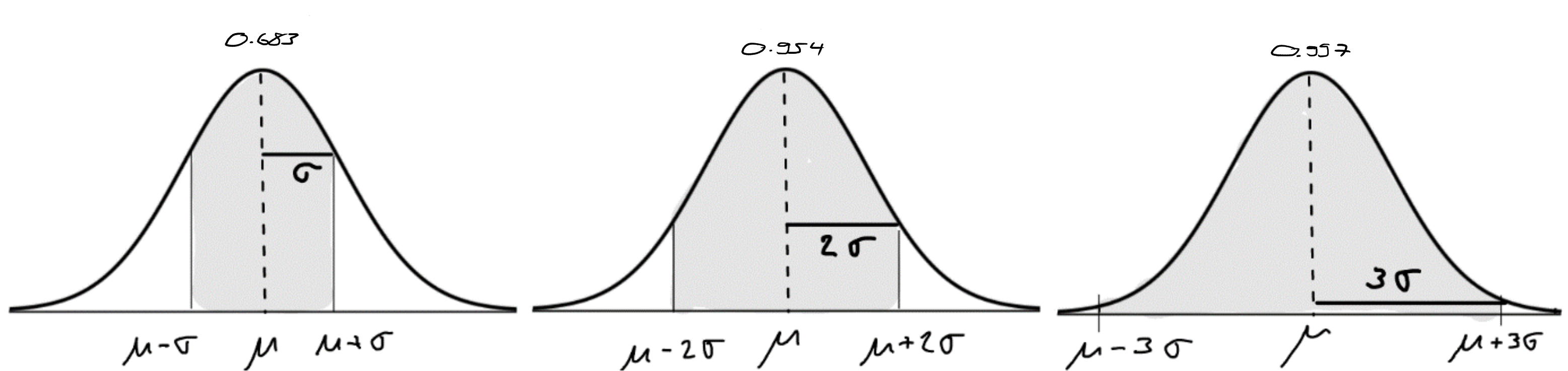
There are some areas under the curve of which are really useful to know. In particular because they occur a lot in statistic applications. Here are some of these areas:
The area under between
- and is
- and is
- and is
Note that these areas are independent of the values of and !
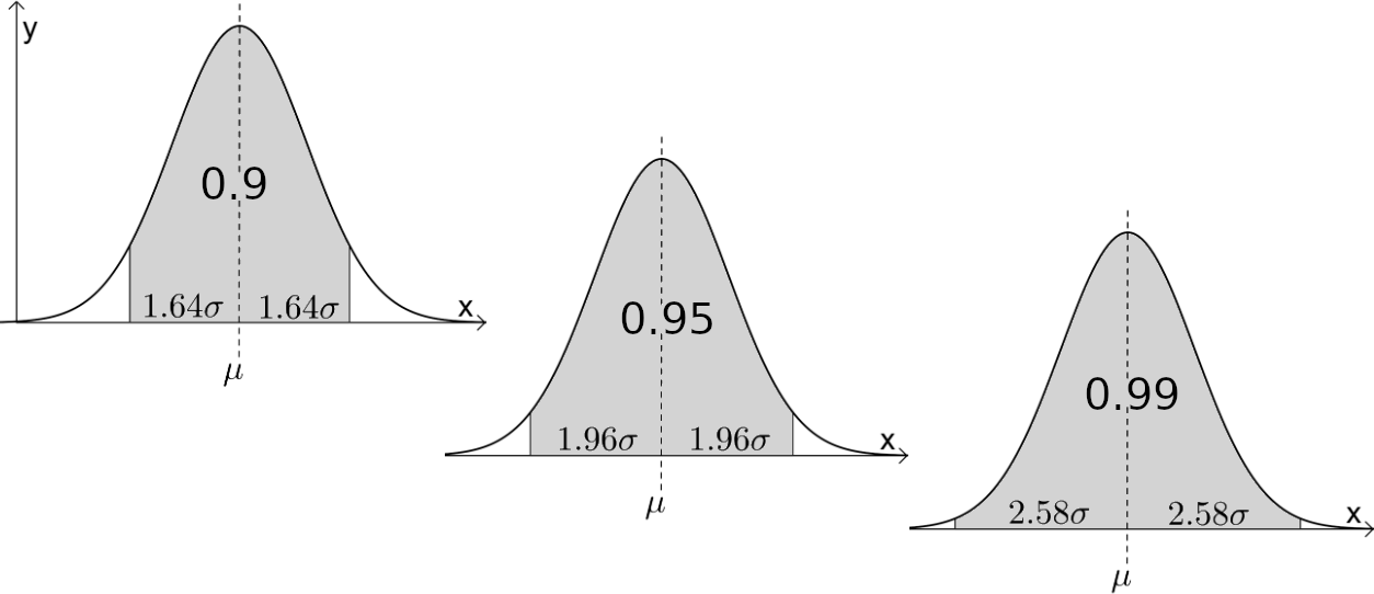
And probably even more useful are the following areas:
The area under between
- and is
- and is
- and is
(see figure below). Note again that these areas are independent of the values of and !
-
Use the calculator to verify the areas in theorem 1 for and (just pick one or two areas, you do not have to verify it for all areas).
-
Consider a random variable with mean and standard deviation which is normally distributed. Determine the following probabilities:
-
The random variable has mean and standard deviation . You perform the experiment times. How many of the outputs of are (roughly) between and ?
Solution
-
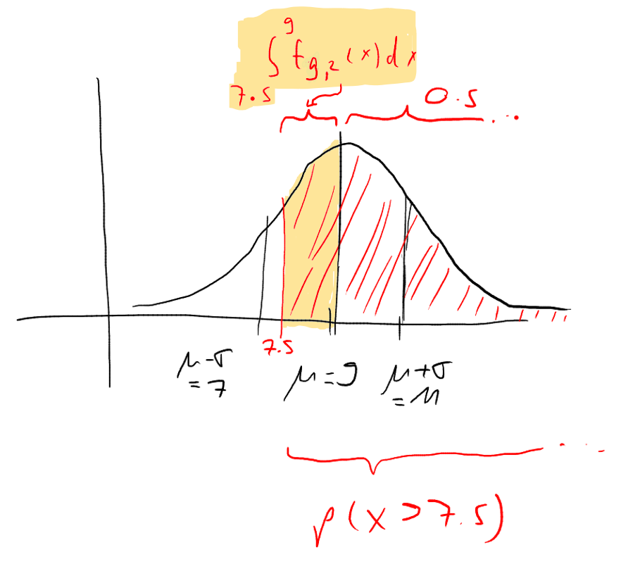
E.g. let's verify that
Because and , we have to show that
So let's calculate the integral
Using the calculator, we get indeed .
-
We try to express the areas using the six areas above, together with the fact that the total area under the curve is .
- (half of the total area of )
- (half of the total area between and , which is )
-
, thus about outputs of .
Q1
A machine produces screws of length . But production is not perfect, and the length my vary. To find out more about it, the length of screws are measured. The frequency table shows the following:
Also calculated from the screws is the mean length, , and the standard deviation, .
- Sketch the histogram of screw lengths based on the table above.
- Check if the screw lengths are approximately normally distributed by drawing the graph of the probability distribution function into the same coordinate system as the histogram. Use the points that were discussed in the previous section. What do you think, are the screws normally distributed?
- Based on the model , determine the probability that the screw length deviates by less than from the mean.
Q2
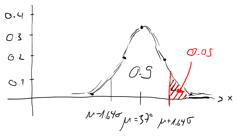
The body temperature of a healthy adult is approximately normally distributed with mean and a standard deviation of .
- Describe the underlying experiment and the random variable .
- Determine the probability, that the temperature deviates by more than from the mean.
- Determine the probability that the temperature is smaller than .
- What minimum temperate do the warmest of the people have?
Q3
The probability density function of a normally distributed random variable has inflection points at and . Determine
- the function equation of
- the probability (use the calculator and integrate numerically)
- the probability (use the calculator and integrate numerically)
Q4
Below is the frequency table of a data set. The mean of the data is , the standard deviation .
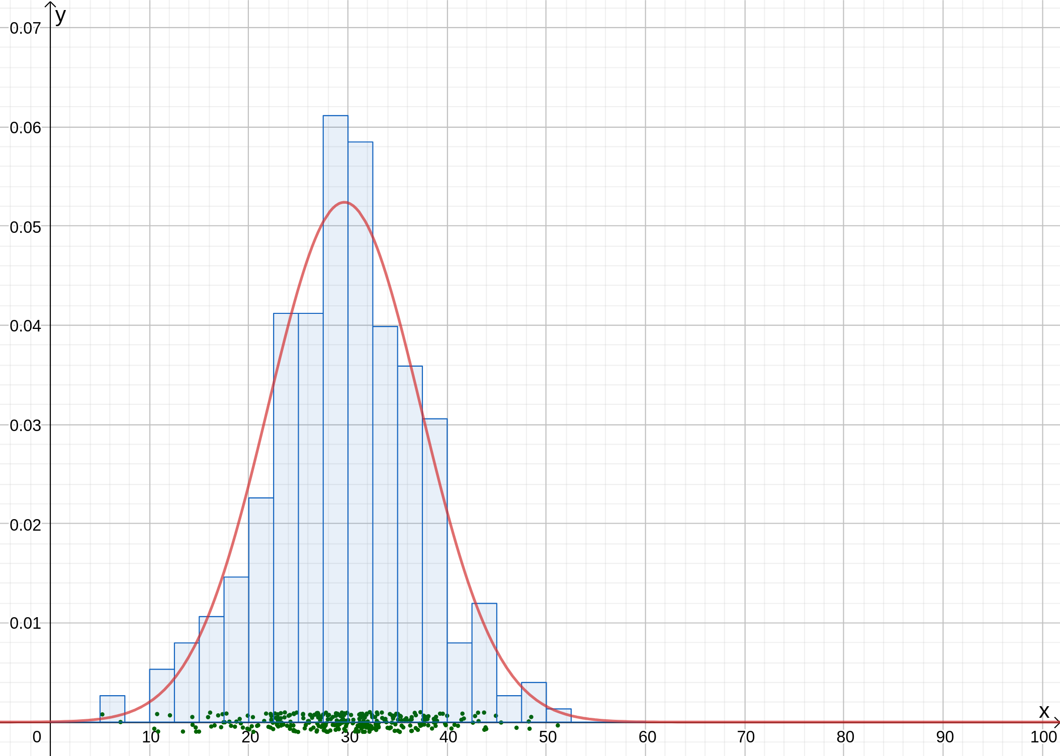
- Show that the data are approximately normally distributed by making the histogram and plotting the normal distribution with parameters and as well.
- Based on the normal distribution, determine the (approximate) probability that a randomly chosen data point lies between and .
- Based on the normal distribution, determine an (approximate) interval such that a randomly chosen data point lies in this interval with probability .
Q5
Measurements of the weight of melons give a mean of and a standard deviation of . The histogram of the weights shows that the weights are approximately normally distributed.
-
Approximately how many melons have a weight greater than ?
-
Between which weights and are about of the melons?
Solution
A1
-
see below
-
see below
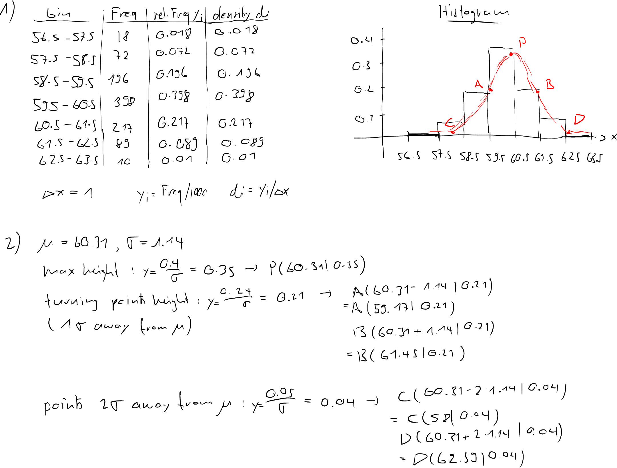
-
As the data (the screw length) is approximately normal distributed (see figure above, in (a)), the probability that the screw length is between and is (see one of the six areas shown at the top). Of course we could also determine the integral using the calculator, and because of and we would find the same number:
A2
-
Random experiment is "select at random a healthy adult", and the random variable is ="measure body temperature".
-
Because , the probability is
and therefore the probability that is outside this range is
-
.
-
The warmest of the people are in the right tail under the curve (see figure below), which corresponds to a minimum temperature of .
A3
-
Find and . Because is in the middle between the -coordinates of the inflection points, we get , and because the inflection points are away from , it is . Thus,
-
and using the calculator, we get
-
Note that we cannot insert into the calculator, so we divide the area as follows (see figure below):
A4
-
To get the densities for the histogram, we have to divide the frequencies by (relative frequency), and then also by the class width . If we add up the frequencies, we get , and the class width is . So we get the densities
The histogram and normal distribution are shown below. For the normal distribution, calculate the points at and as usual. We get the points .
-
It is and . The probability that a data point lies in this interval is the area under the curve of and, and this is (see previous chapter). Of course, we could also use the calculator to work out the integral .
-
It is and
A5
-
Since the data are normally distributed with mean and standard deviation , the norma distribution that approximates the histogram is given by .
The probability that a melon is larger than is the area under the curve of according to . Because , this area is just . So, since there are melons, about melons are heavier than .
-