The normal distribution

We discuss now the most important probability density function. It is used for data that groups around a single value. Here is the definition:

Definition 1

A continuous random variable $X$ is called normally distributed with mean $\mu$ and standard deviation $\sigma$ , if the probability density function of $X$ is

f_{\mu,\sigma}(x)=\frac{1}{\sigma \sqrt{2\pi}}\cdot e^{-\frac{1}{2}\left(\frac{x-\mu}{\sigma}\right)^2}

Note that the mean $\mu$ and the standard deviation $\sigma$ appear in the definition of the density function. Depending on these values (called parameter of the function), the graph of the function will look different.

The simplest case

Let us focus for the moment on the simplest case where $\mu=0$ and $\sigma=1$ ( $\sigma=0$ does not make sense, or at least is not interesting). We then get

f_{0,1}(x)=\frac{1}{\sqrt{2\pi}}\cdot e^{-x^2/2}

which looks like a bell (see below), and for this reason is also called the bell curve.

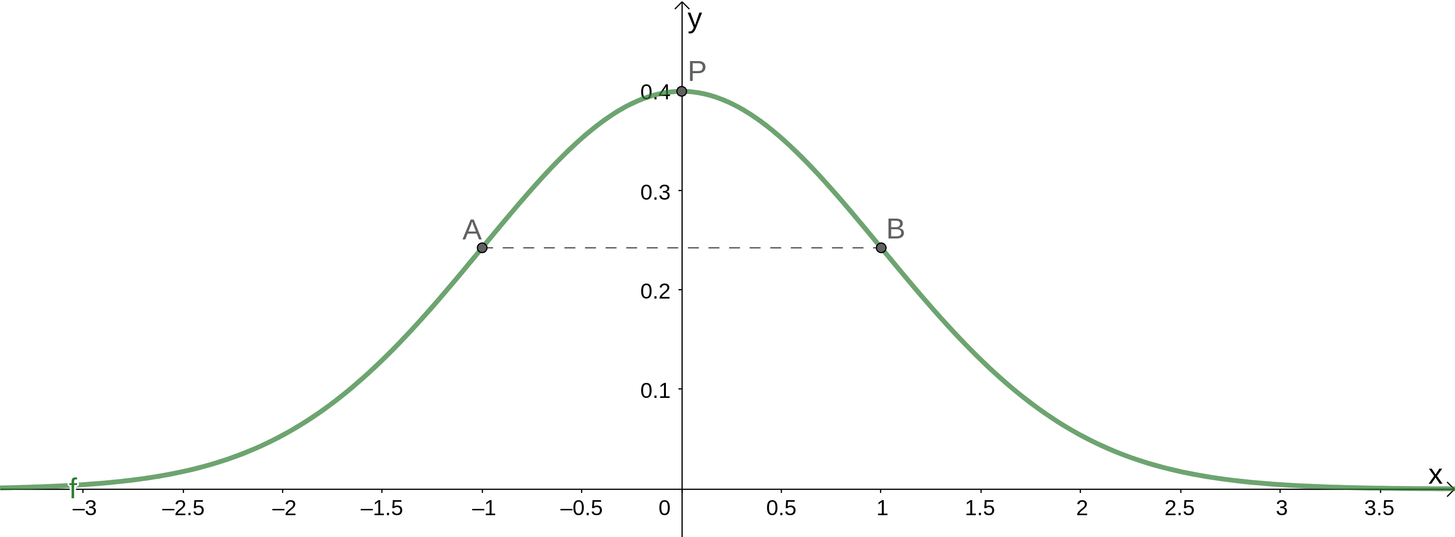
Let's discuss some key features of this graph.

a)

At $x=0$ we get

f_{0,1}(0)=\frac{1}{\sqrt{2\pi}}\cdot e^{0}=\frac{1}{\sqrt{2\pi}}=0.3989... \approx 0.4

which is easily seen on the figure above as well.

b)

To see that $f_{0,1}$ has a maximum at $x=0$ , we can invoke differential calculus. We have to show that $f^{\prime}(0)=0$ and $f^{\prime\prime}(0)<0$ . See the exercise 1 below.

c)

And if we write

f_{0,1}(x)=\frac{1}{\sqrt{2\pi}}\cdot e^{-x^2/2} \approx 0.4\cdot e^{-x^2/2} = \frac{0.4}{e^{x^2/2}}

we see that with $x$ approaching $\infty$ of $-\infty$ , the graph approaches the $x$ -axis, but is always $>0$ .

d)

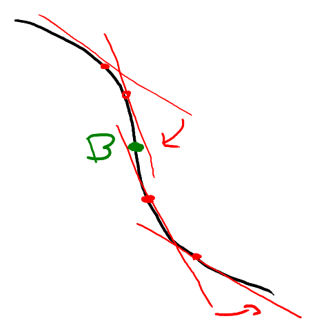
We define the width of the normal distribution as the distance between the inflection points of the graph (indicated above by the points $A$ and $B$ ). Recall that an inflection point is defined as a point on the graph where the slope of the graph changes from increasing to decreasing or vice versa:

Using differential calculus we can show that $A(-1 | 0.24...)$ und $B(1| 0.24...)$ . Thus, the width of the graph $f_{0,1}$ is $2$ (see exercise 1 below).

e)

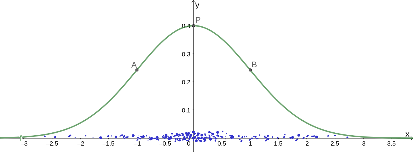
Recall that the probability density function follows the height of the bars in histograms (the density), und therefore is proportional to the relative frequency of the data points in each bin. So we see that the graph of $f_{0,1}$ describes data which is grouped around $\mu=0$ and thins out in both directions.

f)

For $f_{0,1}$ it is

\int_{-\infty}^{\infty} x \cdot f_{0,1}(x)\, dx = 0

(thus, the mean is indeed $\mu=0$ ) and

\sqrt{\int_{-\infty}^{\infty} (x-\mu)^2 \cdot f_{0,1}(x)\, dx} = 1

(the standard deviation is indeed $\sigma=1$ ).

Again, see problem 1 for the proof.

Exercise 1

Show that for $f_{0,1}$ the following is correct:

it has a local maximum at $(0|0.4)$
the inflections points have the coordinates $A(-1 | 0.24)$ and $B(1| 0.24)$
$\int_{-\infty}^{\infty} x \cdot f_{0,1}(x)\, dx = 0$

Solution

Applying the chain rule, we get for the derivative of $f(x)=\frac{1}{\sqrt{2\pi}}\cdot e^{-x^2/2}$ the following:

f'(x)=\frac{1}{\sqrt{2\pi}}\cdot e^{-x^2/2} \cdot (-x)

and for the second derivative we get

f^{\prime\prime}(x)=\frac{1}{\sqrt{2\pi}}\cdot e^{-x^2/2} \cdot (x^2 - 1)

To find the maximum, we have to find an $x$ with
$f'(x)=0$
that is
$f'(x)=\frac{1}{\sqrt{2\pi}}\cdot e^{-x^2/2} \cdot (-x)=0$
and this is only possible for $x=0$ . And because $f^{\prime\prime}(0)<0$ , we are indeed talking about a maximum. The $y$ -coordinate of the peak is
$y=f_{0,1}(0)=\frac{1}{\sqrt{2\pi}}\cdot e^0 \approx 0.4$
Thus we have $P(0|0.4)$
To find the inflection points we have to find $x$ with
$f^{\prime\prime}(x)=0$
Thus find $x$ with
$f^{\prime\prime}(x)=\frac{1}{\sqrt{2\pi}}\cdot e^{-x^2/2} \cdot (x^2 - 1)=0$
we see that this is possible for $x^2-1=0$ , that is, if $x=-1$ or $x=1$ . Using the calculator, we get $y=f(-1)=f(1)=0.24...$ . We thus get $A(-1 | 0.24...)$ and $B(1| 0.24...)$ .

To be sure that these are inflection points, we should also calculate the third derivative and check that $f^{\prime\prime\prime}(1)\neq 0$ and $f^{\prime\prime\prime}(-1)\neq 0$ . This is left to the reader.
We have
$\begin{array}{lll} \int_{-\infty}^{\infty} x \cdot f_{0,1}(x)\, dx &=& \int_{-\infty}^{\infty} x\cdot \frac{1}{\sqrt{2\pi}} e^{-x^2/2}\, dx\\ &=& F(\infty)-F(-\infty)\\ &=& 0 \end{array}$
where $F(x)=-\frac{1}{\sqrt{2\pi}} e^{-x^2/2}$ is the anti-derivative of $x\cdot \frac{1}{\sqrt{2\pi}} e^{-x^2/2}$ .

So the mean is indeed $0$ .

The general case

For the general case the properties are similar. Here they are (without proof):

Theorem 1

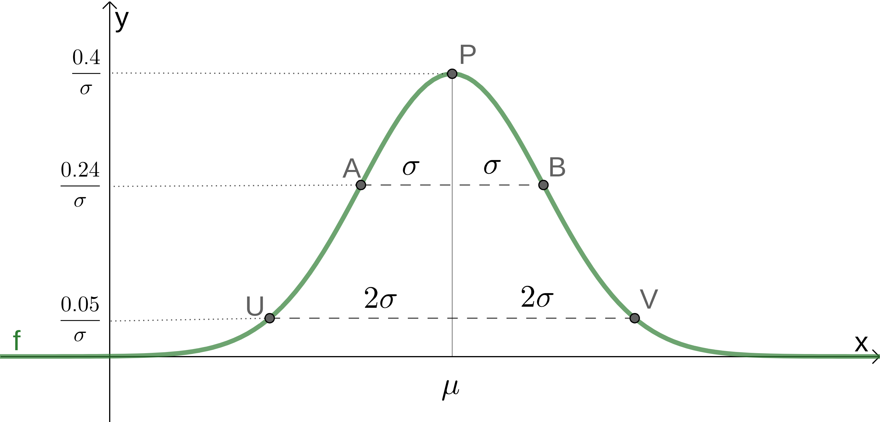
Consider a normally distributed random variable $X$ with mean $\mu$ and standard deviation $\sigma$ . We have the following properties of $f_{\mu,\sigma}$ (see figure below):

the peak $P$ is at $\mu$ , and its height is
$y=f_{\mu,\sigma}(\mu)\approx \frac{0.4}{\sigma}$
the inflection points $A$ and $B$ are one $\sigma$ away from the mean, and have height
$y=f_{\mu,\sigma}(\mu\pm\sigma)\approx\frac{0.24}{\sigma}$
the width is $2\sigma$
The points $U$ and $V$ , which are $2\sigma$ away from $\mu$ , have height
$y=f_{\mu,\sigma}(\mu\pm 2\sigma) \approx \frac{0.05}{\sigma}$
$\int_{-\infty}^{\infty} x \cdot f_{\mu,\sigma}(x)\, dx = \mu$ (the mean of $X$ is $\mu$ )
$\sqrt{\int_{-\infty}^{\infty} (x-\mu)^2 \cdot f_{\mu,\sigma}(x)\, dx} = \sigma$ (the standard deviation of $X$ is $\sigma$ )

So note that $\mu$ tells you where peak of the graph of $f_{\mu,\sigma}$ is along the $x$ -axis, and $\sigma$ tells you how wide the graph is. The larger $\sigma$ is, the flatter will be the graph. This makes sense, as the total area under the graph must be $1$ .

Exercise 2

A random variable $X$ with mean $2$ and standard deviation $0.5$ is normally distributed. Sketch the graph of the density function by first indicating the maximum point $P$ , the inflection points $A$ and $B$ , and the height of the graph $2\sigma$ away from $\mu$ .

To verify the sketch, plot the density function with the calculator (or Geogebra).

Solution

As $\mu=2$ and $\sigma=0.5$ , we have to draw the graph of the function $f_{2,0.5}$ .

The coordinates of the points are

P(2\vert 0.8), A(1.5\vert 0.48), B(2.5\vert 0.48), U(1\vert 0.1), V(3\vert 0.1)