The probability density function
Recall that for a discrete random variable with the values , the list of probabilities
is called the probability function of . It tells you how the probabilities are distributed over the different values of .
We want to define an analogues function for a continuous random variable. Remeber that a continuous the random variable can take on any possible value in a given interval (or even on the whole line ). What exactly this interval is depends on the problem.
Going back to the M&M-Example, the weight could be any value between and , such as or even , but (because of the production process, perhaps) will never go lower than and never exceed . In this case we could choose the interval to be .
However, this poses two problems. First, how do we list the probabilties of a continuous random variable? We cannot form a list as in the discrete case above, because we cannot list all real numbers in an intervall (the real numbers in any interval are not countable).
Back to M&Ms where the interval is . What follows after , is it or , or , or ? I hope you see the problem.
A second problem is that it is for every value that can take on (that is, for every value ). So for the M&Ms, it will be or and so on. Why? It is simply unlikely that several M&Ms have exactly the same weight or , meaning that the relative frequency is always very close to zero. So even if we could list in some way all the probabilities, there would be very little useful information in such a list.
To circumvent these problems, we have to take another approach to capture the probability distribution of a continuous random variable. The basic idea is to replace the probability function of a discrete random variable:
with small intervals for for continous variables:
where the intervals divide the interval . This is just the basic idea. It is not really workable in this version because we do not have a natural way to find the intervals . How big or small do they have to be? How many of them should we choose? In fact we need to approach this problem from a different angle.
We start by defining a new type of function, the so called probability density function of .
Consider a continuous random variable , with values in the interval . The probability density function of , written , is a function with the following properties:
- for all
- for every interval .
or is also possible, that means, intervals like , , or .
In other words, the graph of is never below the -axis, and the probability that takes on a value in the interval is the area beneath the graph of (from to ). See the figure below.
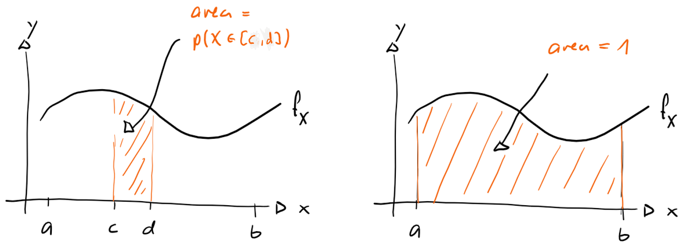
As (as cannot take on any other values, but will always produce a value), the following is valid:
For a probability density function is
That is, the total area beneath the graph of equals .
Every continuous random variable has such a probability density function (apart from some very strange exceptions). Now, the big question is, of course, how do we find for a given random variable . It turns out that the graph of approximately corresponds to the curve formed by the histogram of . To be more precise:
To find the graph of the probability density function of a random variable :
- create a huge number of datapoints drawn from (that is, we repeat the experiment a huge number of times and collect the values of such as the weight of M&Ms)
- create a histogram of the datapoints with a really small bin size
The graph of at any point is then formed by the bar height at :
The more data points are used in the histogram and the smaller is chosen, the better is this approximation.
Proof
Please study the proof, as it helps to understand the issues a bit better.
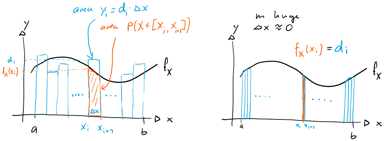
First, consider data points from by repeating the experiment times and let's create a histogram of bin size (figure above left, blue bars). As we have seen in the last chapter, the area of bar is , which is the relative frequency and thus approximately the probability that a data point lands in the bin $x_i,x_{i+1}.
(the more data points we have, the better is this approximation). But from the definition of the probability density function we also know that the area under the curve of between and is exactly (see figure above left, red area):
Thus we have
But because the width of both areas is the same, , we also find that the height of the areas is about the same:
But note that there are many heights in the red area, as it is curved on top. But if we choose really small, all heights will approximately be the same, namely . Thus, we obtain the following result:
And this concludes the proof. Note that there is a more elegant but also a bit more abstract proof, which we quickly show below.
Alternative proof
Let be the antiderivative of , that is, . The bar area in the histogram is, as above
where we used the fundamental theorem of calculus to bring the antiderivative into play. Now, because , we get
and thus
Thus we see again that
Have a look at the proof of this theorem, but also play a bit with the sliders in the geogebra applet below. Observe how the histogram gets smoother and approximates the probability density function for a large number of points and small bin size . Actually, we would need a lot more points and a much smaller bin size to get a really smooth histogram that overlaps exactly with , but you should get the idea.
Open in GeoGebraKnowing the graph of does not necessarily mean we can find its function equation easily. To find such a function equation we often make an educated guess about and then verify our assumption by comparing the histogram with the graph of . But we will not do this here.
-
Argue, why is for every density probability distribution, where takes on values in the interval .
-
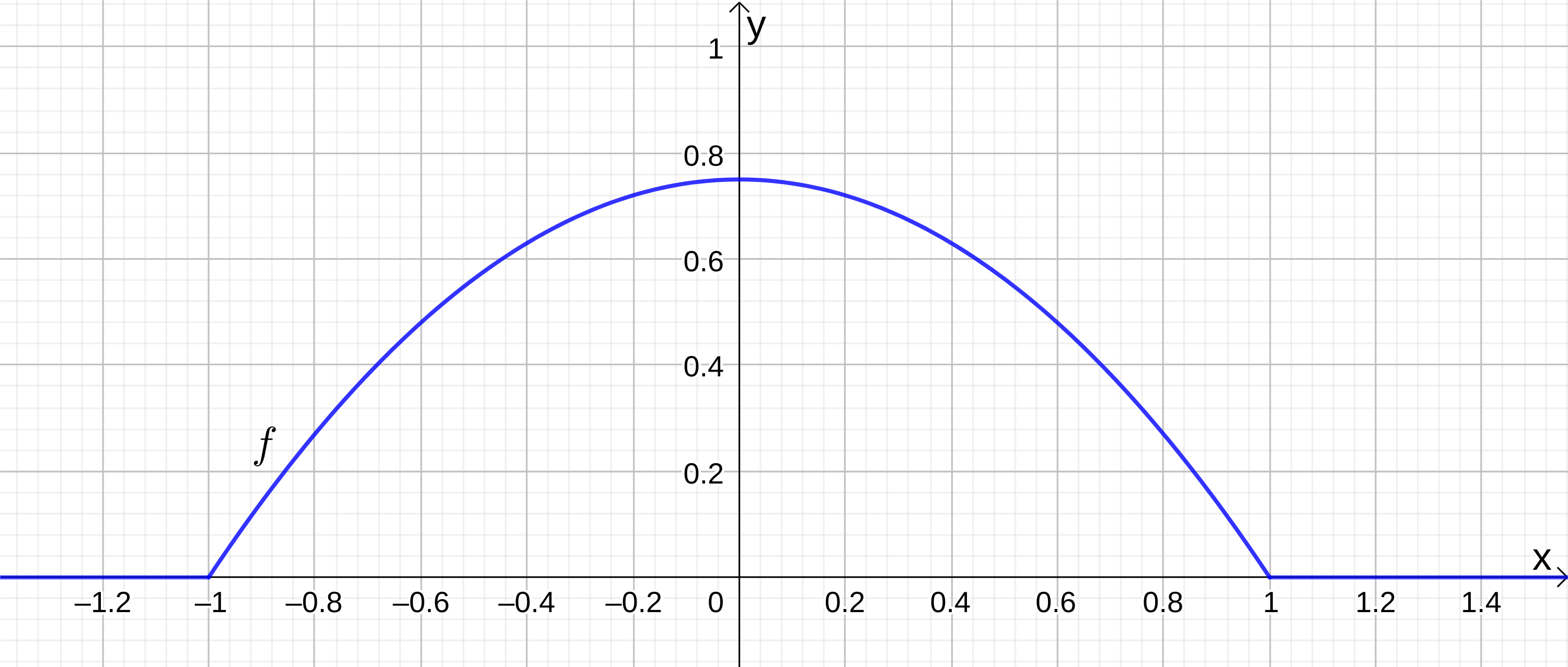
Consider a random experiment with a continuous random variable whose probability density function is
-
Draw the probability density function.
-
Determine the probability that the observed value of is between and , that is, determine the probability .
-
Solution
- .
- . The antiderivative of is
-
The graph is
-
We have
and therefore we have
-