Frequency distribution of continuous data
If the data set is continuous, we cannot simply determine for each possible value how often it occurs. Well, we could, but because all values within a range are possible, most of these values will not be in the dataset, and even if one is, there will probably not be a second or third one.
For example, let's take the continuous data set that results from measuring the weight of M&Ms (in ):
Think of the creation of the M&M's as a random process caused by the machine producing these M&M's. Each M&M will look a bit different, weigh a bit different, and so on due to small imperfections of the machines. So we have the random experiment "produce a M&M", and we use the continuous random variable ="weight of the M&M". We repeat the experiment times to produce the data set above. Clearly, it is highly unlikely that there is a second M&M with the exact weight . So counting all M&M with the weight will not help much for gaining insights into the weight distribution of the data set. It will be a count of , as is for all other M&M in the data set.
A better approach is to ask how many M&M's are in certain range, e.g. from , from , from , and so on. These ranges are called bins, and the width of the range is called the bin size, written (thus ).
So by counting how many M&M's fall into each bin, we might get the following frequency distribution of the data:
For continuous data we are typically interested in the density, which is the relative frequency divided by the bin size, and tells as how densely the data points are arranged in a class:
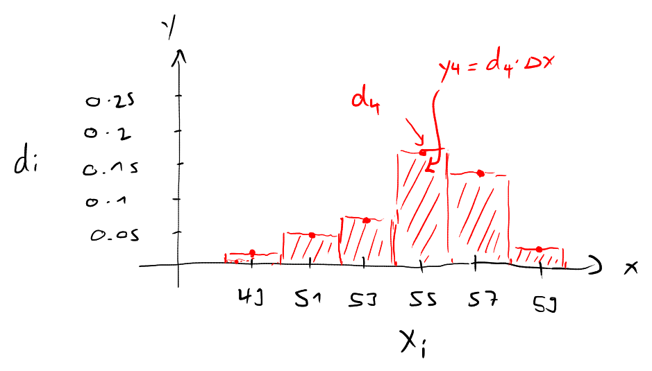
The graphical representation of the relative density is the histogram. In a histogram, the bins are plotted on the vertical axis, and a bar is drawn above the bin with the same width as the bin and the height .
Thus, we have
The area of the bar, , is the relative frequency of the data points in bin :
Warning
In books or websites you can find that the relative frequency in histograms is sometimes represented by the bar height, and the bar area has no meaning at all. In this course, the relative frequency in histograms is always represented by the bar area.
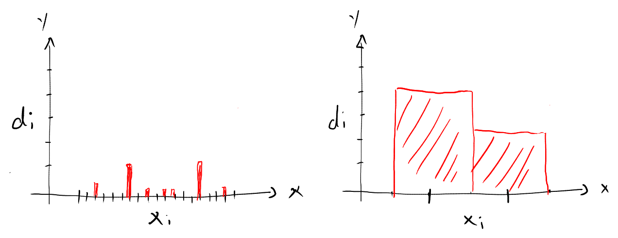
The choice of the bin size is quite important. If we choose the bin-size too small, we will have a lot of bins containing no data, and some which contain perhaps one or two data points (see below, left). If we choose the bin size too big, we lose details about the distribution of the data points (see below, right). So how do we know which bin size to use? Typically, we find the bin size by trial and error - we try out different bin sizes until the resulting histogram is somewhere between these two extremes (see histogram above).
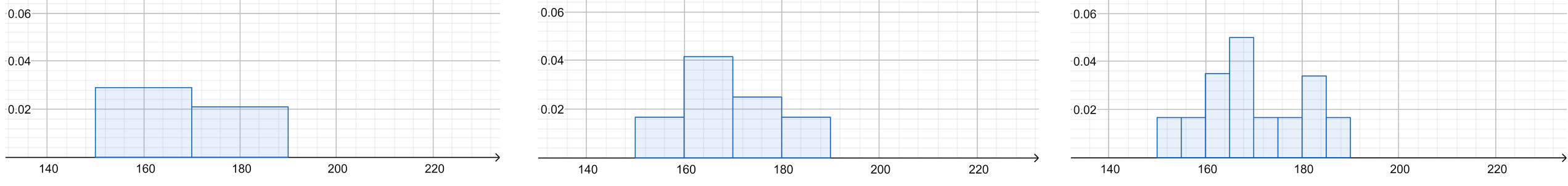
Consider the continuous data set given below (heights of students in ):
Draw three histograms using the bin-sizes given below. Start at and end at .
Show
:
:
:
Returning to our M&M example, recall that we have introduced the continuous random variable "weight of M&M". As is the relative frequency of weights in bin , we have the following:
The area of the bar approximates the probability that will take on a value in bin :
The larger the number of data points in the data set, the better is the approximation.
You bought a huge box of nails and want to know more about the length of these nails (in ). Randomly selecting several hundered nails and measureing its length results in the following histogram:
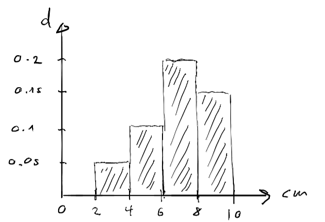
Give an estimate of the following probabilities:
How can you improve the estimate?
Solution
As the bar areas in a histogram are given by the bar are, and the relative frequency approximates the probability, we get
- (bar area above )
- (sum of bar areas above and )
The approximations get better with increasing sample size.