Nudging the input

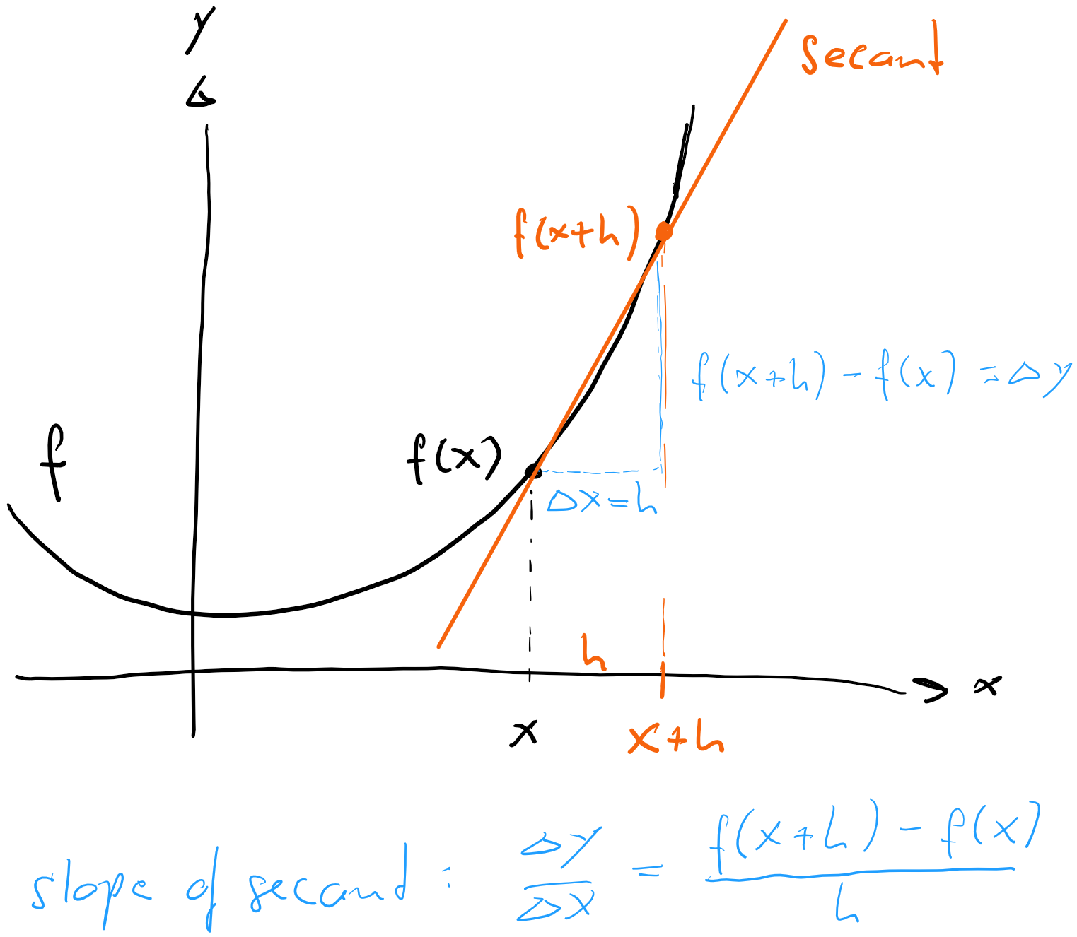
Let's return to the difference quotient, which was the basis for our definition of the derivative:

f'(x)\approx \frac{f(x+h)-f(x)}{h}

Here, think of $x$ as a fixed value, and $h$ can be chosen freely. But the closer $h$ is to zero, the better this approximation will be, and for $h\rightarrow 0$ the $\approx$ sign can be replaced with the $=$ sign.

The geometrical interpretation of this relation is that of slopes. The right-hand side of the equation is the slope of the secant through the points at $x$ and $x+h$ on the graph of $f$ , and for $h\rightarrow 0$ the secant becomes the tangent at $x$ . For this reason, we interpret $f'(x)$ as the slope of the tangent to $f$ at $x$ .

Another useful interpretation of the relation above is obtained by rearranging it a bit: First, multiply both sides by $h$ :

f'(x)\cdot h \approx f(x+h)-f(x)

and then take $f(x)$ on the other side:

\boxed{f(x+h) \approx f(x)+f'(x)\cdot h}

Think again of $x$ as a fixed value, and $h$ can be arbitrary values. And as above, the closer $h$ is to zero, the better will be the approximation. Indeed, for $h=0$ we get a (trivial) equality: $f(x)=f(x)$ .

In order to see what this relation is about, let's go back to our metaphor of functions as little machines, with an input $x$ and an output $y=f(x)$ , and an algebraic rule according which is used to calculate the output from the input (we call this rule the function equation).

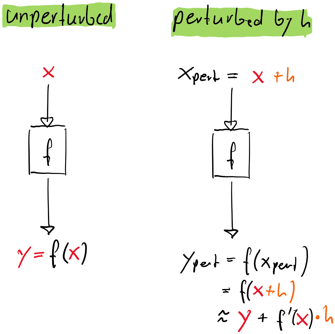
So if $x$ is out fixed value, and we nudge it a little bit to the left or right by a small value $h$ (we call this a perturbation of $x$ by $h$ ), we get a slightly perturbed input $x_{pert}=x+h$ . The output to this perturbed input changes as well. It is now $y_{pert} = f(x_{pert})=f(x+h)$ . So we see that the left side of the relation above is simply the output to the perturbed input $x_{pert}$ . The right side of the relation tells you how this perturbed output relates to the unperturbed output, which is $y=f(x)$ :

\boxed{\underbrace{f(x+h)}_{\text{perturbed}\,\text{output}} \approx \underbrace{f(x)}_{\text{unperturbed}\,\text{ output}}+\underbrace{f'(x)\cdot h}_{\text{size of}\,\text{change}}}

We see now that if I change the input by $h$ , the output changes by $f'(x)\cdot h$ . So $f'(x)$ plays the role of an amplification factor.

Example 1

Consider the machine $f(x)=x^2$ . We want to investigate how the output of the machine reacts to a slight perturbation $h$ of the input $x=3$ .

The amplification factor at $x=3$ is $f'(3)=2\cdot 3=6$ . So any perturbation of input $3$ by $h$ changes the output approximately by $6\cdot h$ .

For example, a perturbation of $h=0.2$ from $x=3$ to $x_{pert}=3.2$ increases the output by approximately $6\cdot 0.2 = 1.2$ , from $y=f(3)=9$ to $y_{pert}\approx 9+1.2=10.2$ .

The actual output is $y_{pert}=f(3.2)=10.24$ .

Exercise 1

Q1

Consider the machine $f(x)=4\ln(x)$ . At what input $x$ is the amplification factor of a perturbation $10$ ?

Q2

You want to build an amplifier (sound) which you then connect with a microphone and speakers. You want your voice to by amplified by a factor of $100$ (that is, $2dB$ ). Find the corresponding machine, that is, find a possible function equation. Assume the perturbation $h$ corresponds to the volume of your voice.

Q3*

Give a proof of the product rule using amplification.

Solution

A1

Find $x$ such that the amplification factor $f'(x)=\frac{4}{x}=10$ . Solving for $x$ , we get $x=\underline{0.4}$ .

A2

You want to find a function $f$ and input $x$ with $f'(x)=100$ . There are of course many possibilities, the simplest is probably $f(x)=\underline{100x}$ , which has a constant amplification of $100$ for any $x$ . Other possibilities are $f(x)=x^{100}$ or $f(x)=50x^2$ and $x=1$ .

A3*

This approach leads to a more intuitive proof of the product rule. So, consider a function $f$ which is the product of two other functions $u$ and $v$ : $f=u\cdot v$ . We want to show that for every $x$ it is

f'(x)=u'(x)v(x)+u(x)v'(x)

We start with the difference quotient for $f$ :

\begin{array}{lll} f'(x) & \approx & \frac{f(x+h)-f(x)}{h}\\ & = & \frac{u(x+h)v(x+h)-u(x)v(x)}{h} \end{array}

Now let us have a closer look at the product $u(x+h)v(x+h)$ : We know now that we can write

u(x+h)\approx u(x)+u'(x)h

v(x+h)\approx v(x)+v'(x)h

and thus

\begin{array}{lll} u(x+h)v(x+h) & \approx & (u(x)+u'(x)h)\cdot (v(x)+v'(x)h)\\ & = & u(x)v(x)+u(x)v'(x)h+u'(x)v(x)h+u'(x)v'(x)h^2\\ \end{array}

Inserting this expression into the difference quotient, we get

\begin{array}{lll} f'(x) & \approx & \frac{f(x+h)-f(x)}{h}\\ & = & \frac{u(x+h)v(x+h)-u(x)v(x)}{h}\\ & \approx & \frac{u(x)v(x)+u(x)v'(x)h+u'(x)v(x)h+u'(x)v'(x)-u(x)v(x)}{h}\\ &=& \frac{u(x)v'(x)h+u'(x)v(x)h+u'(x)v'(x)}{h}\\ &=& \frac{h\cdot (u(x)v'(x)+u'(x)v(x))}{h}+\frac{u'(x)v'(x)h^2}{h}\\ &=& u(x)v'(x)+u'(x)v(x) + u'(x)v'(x)\cdot h \end{array}

If $h\rightarrow 0$ , we see that we get $f'(x)=u(x)v'(x)+u'(x)v(x)+0$ .

q.e.d.

Chaotic dynamical systems

In the machine interpretation of functions, we know now how a small perturbation of the input affects the output: the output changes by an amplified version of the nudge $h$ , where the amplification factor is $f'(x)$ :

f(x+h)=f(x)+f'(x)\cdot h

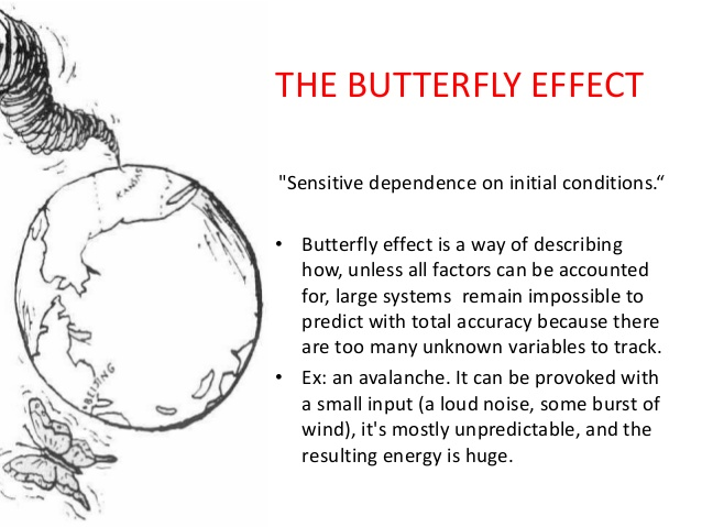
How a small perturbation of the input affects the output of a machine or system is actually a deeply relevant question in many so called dynamical systems. For example, take the weather. The weather can be regarded as a machine or system, where the input is not a single number $x$ , but consists of a huge number of values such as the temperature, atmospheric pressure, etc. on every location on the planet. The output $y=f(x)$ is again an ensemble of many values describing the weather condition anywhere on the planet - where it rains, for how long, how much, and so on.

It turns out that for the weather machine, a small change $h$ in the input can lead to huge changes in the output - this is called the butterfly effect, and is the reason why the weather remains so hard to predict. Such systems are called chaotic.

Even in the case of a complete understanding of the rules according to which the weather machine works (and our understanding is still incomplete), we will have problems predicting the weather. The reason is that we are not able to determine a totally accurate input $x$ (measurement errors, too many variables to measure) and normally work with a slightly inaccurate or perturbed input $x+h$ . And the output can therefore deviate dramatically from the real weather conditions.

The machines we are normally working with, where the output is calculated by applying an algebraic rule to the input, do not behave chaotically. Were the weather behave like one our these machines, a small mistake in wind condition measurements would then perhaps lead to a slightly wrong prediction in the wind conditions, e.g. the weather will be a bit more windy then predicted. But it would not lead to a completely wrong prediction (e.g. a hot summer day instead of a tornado).