Mean and standard deviation of data

Consider a list of data, such as the grades of a student:

4, 6, 3.5, 3, 6

The average or mean value of the grades is obtained by forming the sum of the grades, and dividing by the number of grades:

m = \frac{4+6+3.5+3+6}{5}=4.5

The average value indicates what the typical value is, or the value that "lies somewhere in the middle". The mean value thus calculates a "place" or "position" on the number line, and is therefore also called measure of position. There are several other such measures, e.g. the median, or the quantiles. However, we will not discuss them here.

Another interesting measure expresses how much the data vary. Another student with the same average score of $4.5$ but with a much smaller variance (e.g. five times $4.5$ ) clearly shows a different performance. To qualify such variations in the data, we use the standard deviation. Since the standard deviation measures dispersion, it is also called a measure of dispersion. Again, there are several other measures of dispersion.

The formula for calculation the standard deviation is shown below:

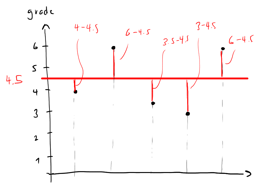
\begin{array}{lll} s &=& \sqrt{\frac{(4-4.5)^2+(6-4.5)^2+(3.5-4.5)^2+(3-4.5)^2+(6-4.5)^2}{5}}\\ &=&\sqrt{1.6}\\ &=&1.26\end{array}

This formula looks complicated, but its meaning is simple enough to understand: it is the average deviation of the data points from the mean (see figure below).

The squared term $(4-4.5)^2$ is the difference between the mean $4.5$ and the data point $4$ , squared. We square it, so that the difference is always positive. So the formula calculates the average of the squared differences between the mean and the data points, and takes the root of this average.

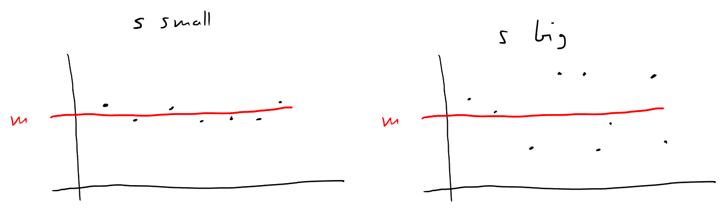
Clearly, a standard deviation $s=0$ means that there is no variation at all, and all data points equal exactly $4.5$ . The bigger $s$ is, the more will the data points deviate from the mean (see figure below).

Some clarifications:

Why do we want to use positive differences only? Because if we simply take the difference, the average of these differences will always be $0$ , although the data points vary wildly about the average (Can you explain why this is true in general?). For example, look at these data points:
$-5, 5, 3$
The mean is
$m = \frac{-5+5+3}{3}=1$
Clearly there is some variation, and indeed the standard deviation is far from zero with
$s=\sqrt{\frac{(-6)^2+4^2+2^2}{3}}=4.32$
However, the average of the difference is zero because some of the differences are positive, others are negative:
$\sqrt{\frac{-6+4+2}{3}}=0$
Why the root? Often data points have units, for example metres. The average is also in metres, and we want the standard deviation also to be in metres. Without taking the root, however, the standard deviation is in square metres, because we square the differences, which are also in metres.

Here is a general definition of the average and the standard deviation:

Definition 1

Consider $n$ data points $x_1, ..., x_n$ . The average or mean value of the data points is

\begin{array}{lll} m &=& \frac{1}{n}\sum_{i=1}^n x_i \\ &=& \frac{x_1+...+x_n}{n} \end{array}

The standard deviation of the data points (from the mean) is

\begin{array}{lll} s &=& \sqrt{\frac{1}{n}\sum_{i=1}^n (x_i-m)^2} \\ &=& \sqrt{\frac{(x_1-m)^2+...+(x_n-m)^2}{n}} \end{array}

The variance of the data points is the squared standard deviation: $v=s^2$

Exercise 1

Determine the mean, standard deviation and variance of the data points
$30, 43, 21.2, 0$
Consider $1000$ melons, of which $20\%$ have weight $3.2 kg$ , $50\%$ have weight $3.5 kg$ , and the remaining $30\%$ have weight $4.1 kg$ . Determine the mean weight and the standard deviation.

Solution

$m=23.55, s=15.65, v=245$
$200$ melons have weight $3.2 kg$ , $500$ melons have weight $3.5 kg$ , and $300$ melons have weight $4.1 kg$ . So we have
$\begin{array}{lll} m &=& \frac{200\cdot 3.2 + 500\cdot 3.5 + 300\cdot 4.1}{1000}\\ &=& \frac{200\cdot 3.2}{1000} + \frac{500\cdot 3.5}{1000} + \frac{300\cdot 4.1}{1000}\\ &=& 0.2\cdot 3.2 + 0.5\cdot 3.5 + 0.3\cdot 4.1\\ &=& \underline{3.62 kg}\\ s &=& \sqrt{\frac{200\cdot (3.2-3.62)^2+500\cdot (3.5-3.62)^2+300\cdot (4.1-3.62)^2}{1000}}\\ &=& \sqrt{\frac{200\cdot (3.2-3.62)^2}{1000}+\frac{500\cdot (3.5-3.62)^2}{1000}+\frac{300\cdot (4.1-3.62)^2}{1000}}\\ &=& \sqrt{0.2\cdot (3.2-3.62)^2+ 0.5\cdot (3.5-3.62)^2 + 0.3\cdot (4.1-3.62)^2}\\ &=& \underline{0.334 kg} \end{array}$

The solution of the second exercise 1.2 highlights an interesting insight, which will be important in the next chapter: If many of the data points are equal, we can use the percentages of equal data points to calculate $m$ and $s$ very easily. In fact, we do not even have to know the total number of data points. Here is an example.

Example 1

Assume that $35\%$ of the data points have the value $7.1$ , and the remaining $65\%$ of the data points have the value $9$ . The mean and the standard deviation of the data points are:

m=0.35\cdot 7.1 + 0.65\cdot 9=8.335

s=\sqrt{0.35\cdot (7.1-8.335)^2 + 0.65\cdot (9-8.335)^2}=0.90624

Do you understand why? Uncollapse to see the explanation.

Solution

Let as assume that there are $n$ data points (e.g. $n=1000$ ). There are $0.35 n$ data points with value $7.1$ and $0.65 n$ data points with value $9$ . There are also $0.35n$ squared differences $(7.1-m)^2$ and $0.65n$ squared differences $(9-m)^2$ . Thus

\begin{array}{lll} m &=& \frac{0.35n \cdot 7.1 + 0.65n\cdot 9}{n}\\ &=& \frac{0.35\cdot n\cdot 7.1}{n} + \frac{0.65\cdot n\cdot 9}{n}\\ &=& 0.35\cdot 7.1+0.65\cdot 9\\ &=& 8.335\\ s &=& \sqrt{\frac{0.35n \cdot (7.1-m)^2 + 0.65n\cdot (9-m)^2}{n}}\\ &=& \sqrt{\frac{0.35\cdot n\cdot (7.1-8.335)^2}{n} + \frac{0.65\cdot n\cdot (9-8.335)^2}{n}}\\ &=& \sqrt{0.35\cdot (7.1-8.335)^2 + 0.65\cdot (9-8.335)^2}\\ &=& 0.906 \end{array}