The probability function of RVs

We start with the definition of the probability distribution.

Definition 1

Consider a random variable $X$ of a random experiment, where $X$ can take on the possible (output) values $x_1, ..., x_r$ . The set of probabilities

p(X=x_1), ..., p(X=x_r)

is called the probability function of $X$ . This because we can think of $f_X(x_i)= p(X=x_i)$ as a function with input values $x_1, ...,x_r$ and output values $p(X=x_1), ... p(X=x_r)$ .

The function

F_X(x)=p(X\leq x)

where the input $x$ is a real number is called the cumulative distribution function of $X$ . $F_X(x)$ is the probability that the random variable $X$ takes on a value of $x$ or smaller. That is, it is the probability, that an output of the experiment has the value $\leq x$ .

Warning

Some books refer to the probability function as a probability distribution or probability density function, and to the cumulative disitribution function as a distributuion function. So stay flexible ... .

We often draw the probability function in a coordinate system, where the values $x_1, ..., x_r$ are indicated along the $x$ -axis, and the probabilities $p(X=x_1), ..., p(X=x_r)$ along the $y$ -axis. For the cumulative distribution function we draw, as always for functions, the input $x$ along the $x$ -axis and the output $p(X=x)$ along the $y$ -axis. Here is an example:

Exercise 1

A fair coin is flipped twice. The random variable is $N$ ="number of heads".

Determine the probability function of $N$ , and draw the function in a coordinate system.
Draw the cumulative distribution function $F_N$ .

Solution

The possible values of $N$ are $\{0,1,2\}$ , where

\begin{array}{lll} N=0 &=& \{TT\}\\ N=1&=&\{TH,HT\}\\ N=2&=&\{HH\} \end{array}

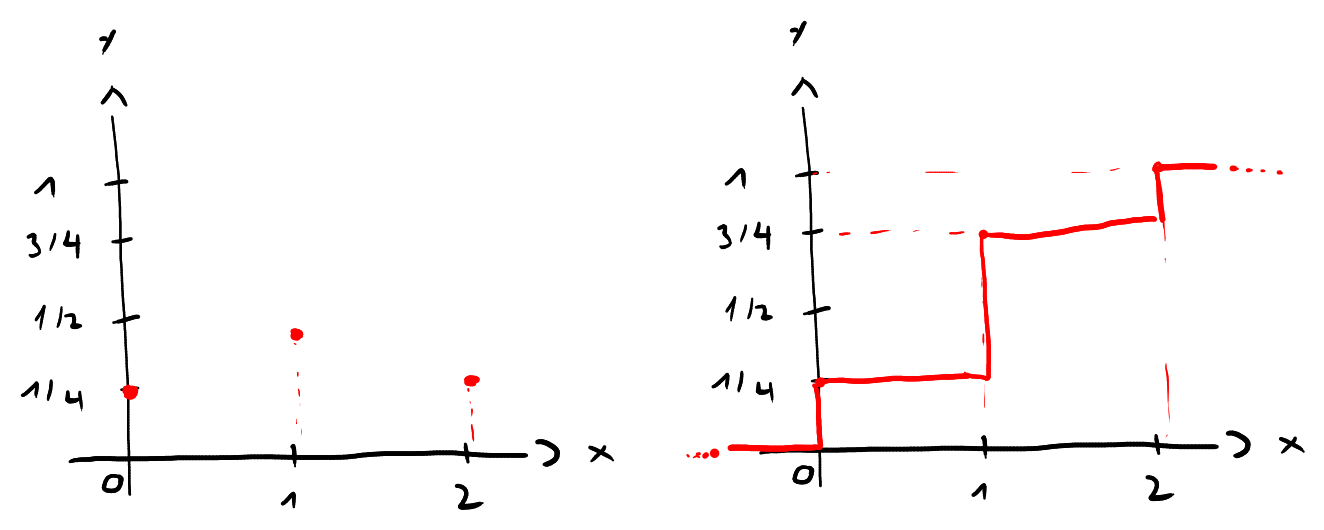
As this is a Laplace experiment, we have the following probability function of $N$ :

\begin{array}{lll} p(N=0) &=& \frac{1}{4}\\ p(N=1)&=&\frac{2}{4}\\ p(N=2)&=&\frac{1}{4} \end{array}

(see figure below, left).

The cumulative distribution function $F_N(x)$ is the probability that the number of heads is equal or less than $x$ . For example,

\begin{array}{lll} F_N(0) &=& \frac{1}{4}\\ F_N(0.5) &=& \frac{1}{4}\\ F_N(1)&=&\frac{3}{4}\\ F_N(1.5)=&=&\frac{3}{4}\\ F_N(2)&=&\frac{4}{4}\\ F_N(2.5)&=&\frac{4}{4}\\ \end{array}

and so on. It is a staircase function, where the jumps occur at the values $x=0, 1$ and $2$ . See the figure below, right.

As the events $X=x_1, ... X=x_k$ are pairwise mutually exclusive, and actually form a partition of the sample space $S$ , we have the following important properties:

Theorem 1

Consider the probability function $p(X=x_1), ..., p(X=x_r)$ of a random variable $X$ . We have the following:

For arbitrary values of $X$ , e.g. $x_1, x_2$ and $x_3$ it is
$p(X=x_1 \cup X=x_2 \cup X=x_3) = p(X=x_1)+p(X=x_2)+p(X=x_3)$
The sum of all probabilities of the probability function is $1$ :
$\sum_{k=1}^r p(X=x_k)=p(X=x_1)+...+p(X=x_r)=1$
$F_X(x)$ is the sum of all probabilities $p(X=x_k)$ with $x_k\leq x$ . Thus, if for a given $x$ exactly the values $x_1, x_2, x_3\leq x$ , then
$F_X(x)=p(X=x_1)+p(X=x_2)+p(X=x_3)$

Proof

The proof is straight forward.

This follows from the fact that the events are pairwise mutually exclusive.
Follows from statement 1, and the fact that the union of all those events form the sample space $S$ , so we have
$\begin{array}{lll} 1 &=& p(S)\\ &=& p(X=x_1\,\cup\, ... \,\cup\, X=x_r)\\ &=& p(X=x_1)+...+p(X=x_r)\\ \end{array}$
Follows from statement $1$ .

Exercise 2

A fair die is rolled twice. Consider the random variable $S$ ="sum of the two numbers".

Determine the possible values of $S$ .
Determine and draw the probability function of $S$ .
Determine $F_S(4)$
Draw the graph of $F_S$ .

Solution

The sample space is

\begin{array}{l|ccccccc} + & 1 & 2 & 3 & 4 & 5 & 6 \\\hline 1 & 2 & 3 & 4 & 5 & 6 & 7 \\ 2 & 3 & 4 & 5 & 6 & 7 & 8 \\ 3 & 4 & 5 & 6 & 7 & 8 & 9 \\ 4 & 5 & 6 & 7 & 8 & 9 & 10 \\ 5 & 6 & 7 & 8 & 9 & 10 & 11 \\ 6 & 7 & 8 & 9 & 10 & 11 & 12 \\ \end{array}

Possible outputs of $S$ : $\{ 2,3,4,..., 11, 12\}$
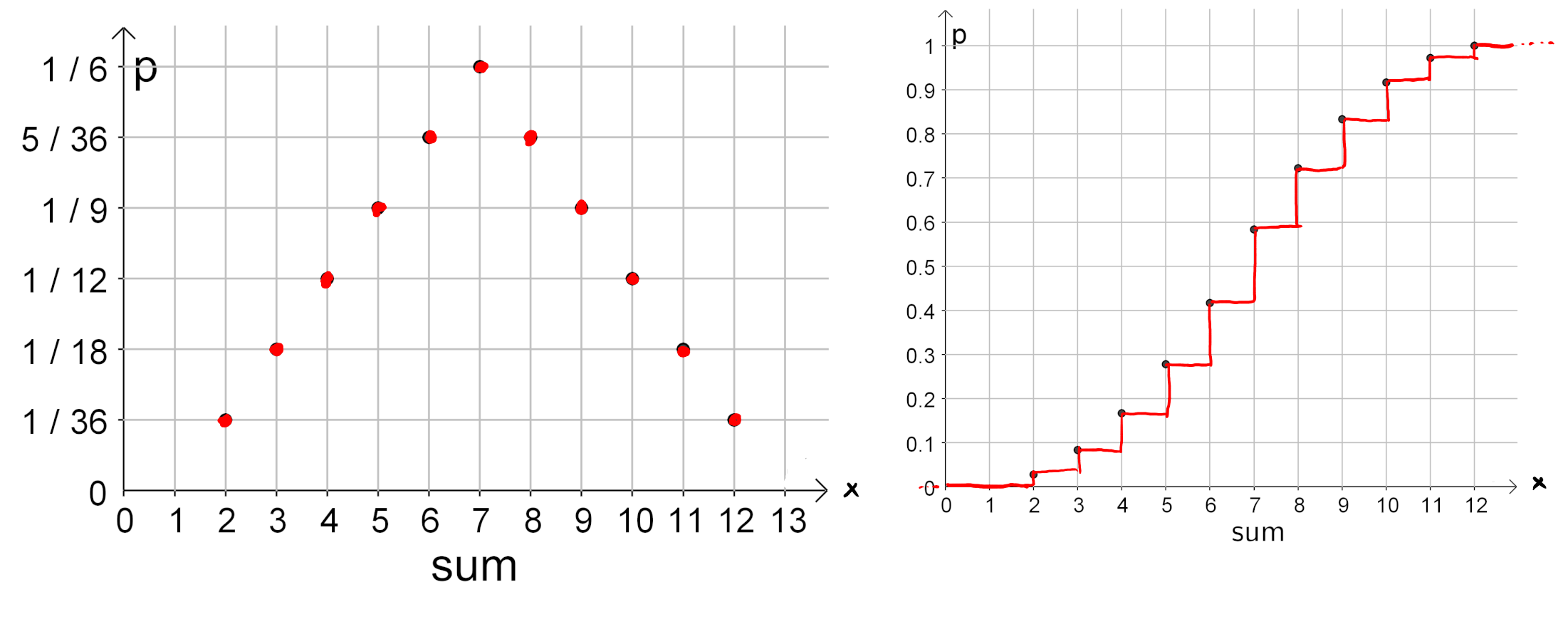
The probability function is (for a figure see below)
$\begin{array}{lll} p(S=2)&=&\frac{1}{36}\\ p(S=3)&=&\frac{2}{36}\\ p(S=4)&=&\frac{3}{36}\\ p(S=5)&=&\frac{4}{36}\\ p(S=6)&=&\frac{5}{36}\\ p(S=7)&=&\frac{6}{36}\\ p(S=8)&=&\frac{5}{36}\\ p(S=9)&=&\frac{4}{36}\\ p(S=10)&=&\frac{3}{36}\\ p(S=11)&=&\frac{2}{36}\\ p(S=12)&=&\frac{1}{36} \end{array}$
We have
$\begin{array}{lll} F_S(4)&=&p(S\leq 4)\\ &=&p(S=2)+p(S=3)+p(S=4)\\ &=&\frac{6}{36}=\frac{1}{6} \end{array}$
The graph of $F$ is shown below. It helps to calculate the points of the graph where it jumps:
$\begin{array}{lll} F_S(2)&=&\frac{1}{36}\\ F_S(3) &=&\frac{3}{36}\\ F_S(4)&=&\frac{6}{36}\\ F_S(5)&=&\frac{10}{36}\\ F_S(6)&=&\frac{15}{36}\\ F_S(7)&=&\frac{21}{36}\\ F_S(8)&=&\frac{26}{36}\\ F_S(9)&=&\frac{30}{36}\\ F_S(10)&=&\frac{33}{36}\\ F_S(11)&=&\frac{35}{36}\\ F_S(12)&=&\frac{36}{36}=1\\ \end{array}$

Exercise 3

The probabilities $p(X=1)=x^2$ , $p(X=2)=3x$ , $p(X=3)=0.1$ form the probability function of a random variable $X$ . Determine the value $x$ and the probabilities.

Solution

As $p(X=1)+p(X=2)+p(X=3)=1$ , it follows

x^2+3x+0.1=1

Solve for $x$ (midnight formula), we get $x_1=-3.27$ and $x_2=0.275$ . As probabilities $<0$ are not possible, we have to exclude $x_1$ from the solutions. So $p(X=1)=\underline{0.076}$ , and $p(X=2)=\underline{0.824}$ .