Approximating the integral

While our goal is to find the exact value of an integral, let's start with a less ambitious goal by simply approximate it reasonably well. Let's discuss the method we use with the integral shown below:

Recipe 1

Consider the integral

0.14f(x)dx\int_{0.1}^4 f(x)\, dx

where f(x)=14x2+12f(x)=\frac{1}{4} x^2+\frac{1}{2}

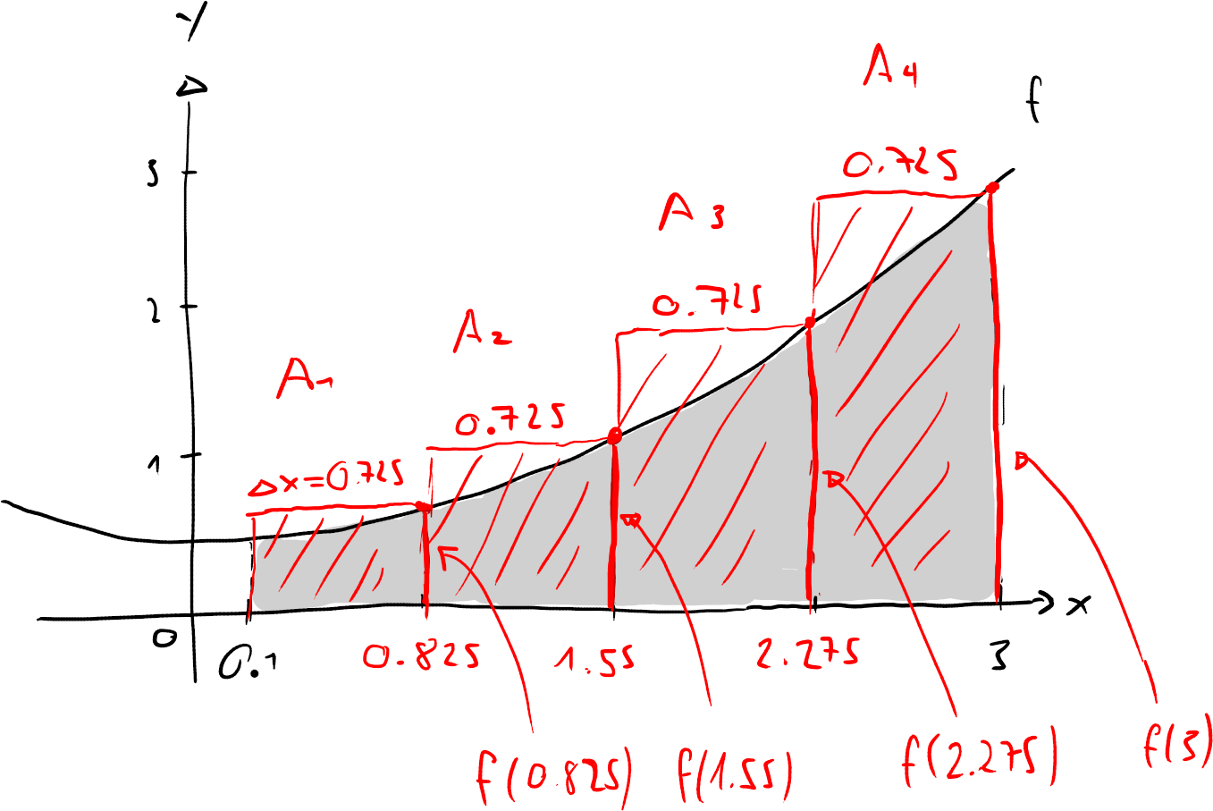
In the example above we used n=4n=4 bars. If A1,A2,A3A_1, A_2, A_3 and A4A_4 are the areas of each bar, we see that sum of these bar areas approximates the integral

0.13f(x)dk=14Ak=A1+A2+...+A4\int_{0.1}^3 f(x)\, d \approx \sum_{k=1}^4 A_k = A_1+A_2+...+A_4

Any other number of bars nn is also okay, and intuitively it should be clear that the more bars we take, the better the approximation will be (see next chapter for a discussion of this). Observe how we draw the bars, which also gives them their width and height:

  1. Each bar starts on the xx-axis, and has equal width, which we typically denote by Δx\Delta x.
  2. Calculating the bar width Δx\Delta x: As the n=4n=4 bars have to span the segment from a=0.1a=0.1 to b=3b=3, it has to be Δx+Δx+Δx+Δx=30.1\Delta x+\Delta x +\Delta x+ \Delta x = 3-0.1 and thus 4Δx=30.14\cdot \Delta x=3-0.1 It follow Δx=30.14=0.725\Delta x=\frac{3-0.1}{4}=0.725
  3. Calculating the right edge position of each bar: The height of each bar is defined by its right edge, we furst need to find out where those right edges start on the xx-axis. Let's denote those positions by x1,x2,x3x_1, x_2, x_3 and x4x_4. As the first bar starts at a=0.1a=0.1, and each bar has width Δx=0.725\Delta x=0.725, we see that the positions are x1=0.1+1Δx=0.1+10.725=0.825x2=0.1+2Δx=0.1+20.725=1.55x3=0.1+3Δx=0.1+30.725=2.275x4=0.1+4Δx=0.1+40.725=3\begin{array}{lllll} x_1 &=& 0.1+1\cdot\Delta x &=& 0.1+1\cdot 0.725 = 0.825\\ x_2 &=& 0.1+2\cdot\Delta x &=& 0.1+2\cdot 0.725 = 1.55\\ x_3 &=& 0.1+3\cdot\Delta x &=& 0.1+3\cdot 0.725 = 2.275\\ x_4 &=& 0.1+4\cdot\Delta x &=& 0.1+4\cdot 0.725 = 3 \end{array}
  4. Calculating each bar area: The bar area is bar width times bar height, where the height can be calcultated using the function ff. Thus, we have A1=f(0.825)Δx=0.670.725=0.485A2=f(1.55)Δx=1.100.725=0.798A3=f(2.275)Δx=1.790.725=1.300A4=f(3)Δx=2.250.725=1.994\begin{array}{llll} A_1 &=& f(0.825)\cdot \Delta x &=& 0.67 \cdot 0.725=0.485\\ A_2 &=& f(1.55)\cdot \Delta x &=& 1.10 \cdot 0.725=0.798\\ A_3 &=& f(2.275)\cdot \Delta x &=& 1.79 \cdot 0.725=1.300\\ A_4 &=& f(3)\cdot \Delta x &=& 2.25 \cdot 0.725=1.994\\ \end{array}

Thus, a reasonable approaximation is

0.14f(x)dx0.485+0.798+1.3+1.994=4.577\int_{0.1}^4 f(x)\, dx \approx 0.485+0.798+1.3+1.994=4.577

Let's summarise all this for general bar numbers.

Theorem 1

Any integral can be approximated by a sum of nn bars or equal width

Equation 1
abf(x)dxk=1nf(xk)Δx\int_a^b f(x)\, dx \approx \sum_{k=1}^n f(x_k)\Delta x

Integral approximated by the Rieman sum, using the sigma notation.

or without the sigman notation

Equation 2
abf(x)dxf(x1)Δx++f(xn)Δx\int_a^b f(x)\, dx \approx f(x_1)\Delta x + \dots +f(x_n)\Delta x

Integral approximated by the Rieman sum, without using the sigma-notation.

where

  • Δx=ban\Delta x =\frac{b-a}{n} is the bar width
  • x1,...,xnx_1,...,x_n are the positions of the right edges of the bars, that is, x1=a+Δx,x2=1+2Δx,,xn=a+nΔx=bx_1=a+\Delta x, x_2=1+2\Delta x, \dots, x_n=a+n\Delta x = b
  • f(x1),,f(xn)f(x_1),\dots,f(x_n) are the bar heights
  • A1=f(x1)Δx,,An=f(xn)ΔxA_1=f(x_1)\Delta x,\dots, A_n=f(x_n)\Delta x are the bar areas

The sum of bar areas is also called the Riemann sum.

Note 1

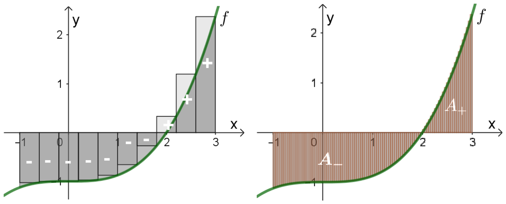
The sum of bars (Rieman sum) actually approximate signed areas, not normal areas, which is good news for us, as integrals are defined as signed areas. To see why, observe the figure below, in the region on the xx-axis where the graph ff goes below the xx-axis. The following is true for this region:

  • A bar has to be drawn downwards, as the bar is always from the xx-axis to the graph.
  • Because f(x)0f(x)\leq 0 for an xx in this region, we also have that the bar area f(x)Δx0f(x)\Delta x\leq 0. That is, the bars count negative as soon as the graph goes below the aaxis.
Exercise 1
  1. Use nn bars to approximate the integrals below. Always create a figure and indicate the bars accurately. For (a)-(c) also calculate the exact integral using basic geometry, and compare.

    1. 0.543dx\int_{0.5}^4 3\, dx, use n=7n=7 bars (we integrate over the contant function f(x)=3f(x)=3 for all xx).
    2. 0.540.5x+1dx\int_{0.5}^4 0.5x+1\, dx, use n=4n=4 bars.
    3. 111x2dx\int_{-1}^1 \sqrt{1-x^2}\, dx, use n=5 bars (we integrate over the half circle of radius 11 with center at coordinate origin).
    4. 02x2dx\int_0^2 x^2\, dx, use n=3n=3 bars.
    5. 122xdx\int_1^2 \frac{2}{x}\,dx, use n=2n=2 bars.
  2. Use 100100 bars to approximate 01x2dx\int_0^1 x^2\, dx.

    Hint: You need the formula for summing the first nn square numbers, see last exercise in the sigma-notation chapter.

  3. A car moves along a straight line. The instantaneous speed at time xx can be described by some function f(x)f(x). We approximate the area from time aa to time bb beneath the graph of ff using nn bars. In this context, what is the meaning of the sum of bar areas

    k=1nf(xk)Δx\sum_{k=1}^n f(x_k)\Delta x

    So what is the integral actually calculating in physics terms?

Solution
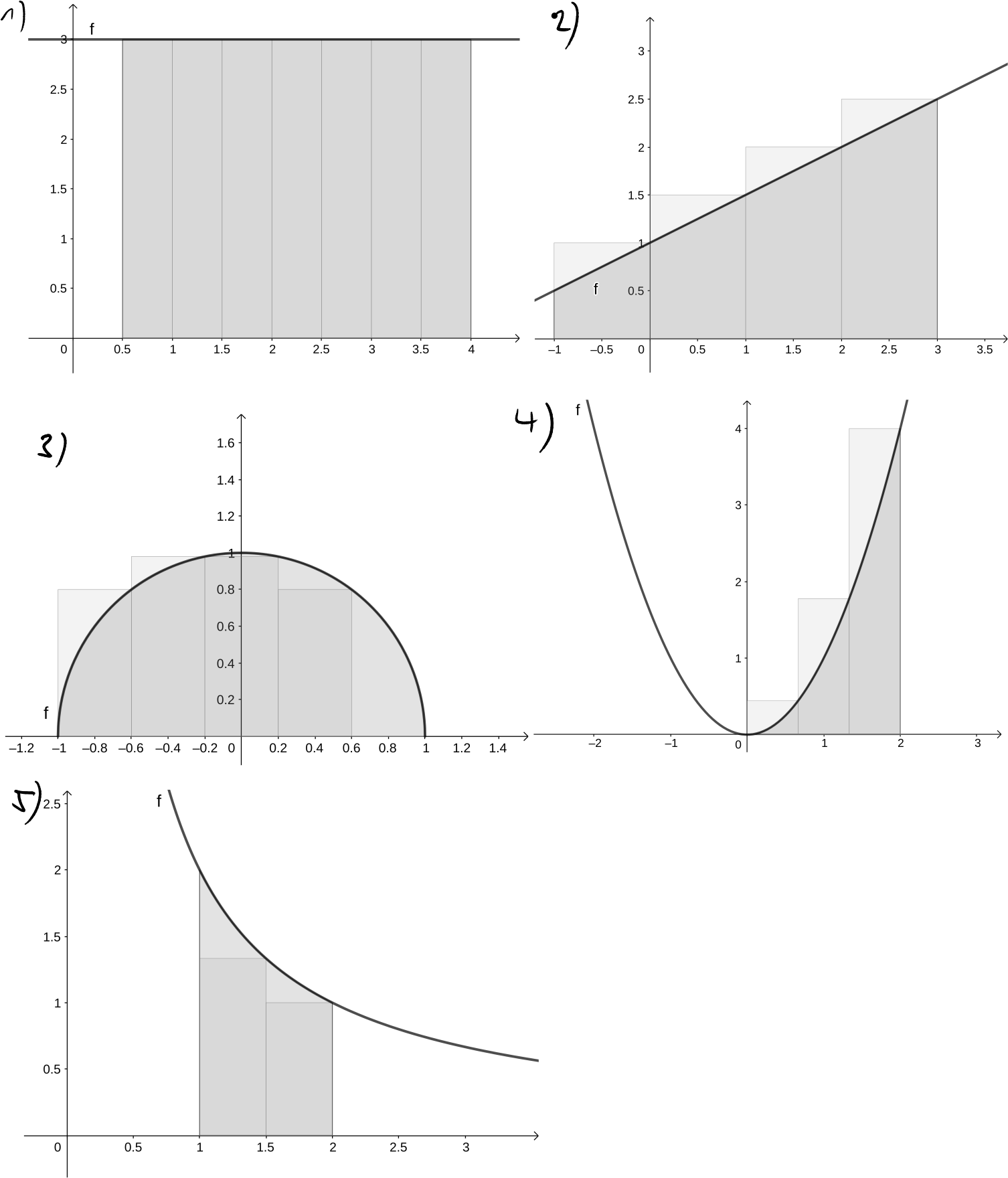
  1. The graphs are shown below.
    1. Δx=40.57=0.5\Delta x =\frac{4-0.5}{7}=0.5 x1=1,x2=1.5,x3=2,x4=2.5,x5=3,x6=3.5,x7=4x_1=1, x_2=1.5, x_3=2, x_4=2.5, x_5=3, x_6=3.5, x_7=4 k=17f(xk)Δx=f(1)0.5+f(1.5)0.5+...+f(4)0.5=1.5+1.5+1.5+1.5+1.5+1.5+1.5=10.5\begin{array}{lll} \sum_{k=1}^7 f(x_k)\Delta x & = f(1)\cdot 0.5+ f(1.5)\cdot 0.5+...+f(4)\cdot 0.5\\ & = 1.5+1.5+1.5+1.5+1.5+1.5+1.5\\ & = \underline{10.5}\\ \end{array} Af=3.53=10.5A_f=3.5\cdot 3=\underline{10.5} (see exercise in previous section)
    2. Δx=3(1)4=1\Delta x =\frac{3-(-1)}{4}=1 x1=0,x2=1,x3=2,x4=3x_1=0, x_2=1, x_3=2, x_4=3 k=14f(xk)Δx=f(0)1+f(1)1+f(2)1+f(3)1=1+1.5+2+2.5=7\begin{array}{lll} \sum_{k=1}^4 f(x_k)\Delta x & = f(0)\cdot 1+ f(1)\cdot 1+f(2)\cdot 1+f(3)\cdot 1\\ & =1+1.5+2+2.5\\ & =\underline{7}\\ \end{array} Af=6A_f=\underline{6} (see exercise in previous section).
    3. Δx=1(1)5=0.4\Delta x =\frac{1-(-1)}{5}=0.4 x1=0.6,x2=0.2,x3=0.2,x4=0.6,x5=1x_1=-0.6, x_2=-0.2, x_3=0.2, x_4=0.6, x_5=1 k=15f(xk)Δx=f(0.6)0.4+f(0.2)0.4+f(0.2)0.4+f(0.6)0.4+f(1)0.4=0.32+0.39+0.39+0.32+0=1.42\begin{array}{lll} \sum_{k=1}^5 f(x_k)\Delta x & = f(-0.6)\cdot 0.4+ f(-0.2)\cdot 0.4+f(0.2)\cdot 0.4+f(0.6)\cdot 0.4+f(1)\cdot 0.4\\ & = 0.32+0.39+0.39+0.32+0\\ & =\underline{1.42}\\ \end{array} Af=π2=1.57...A_f=\frac{\pi}{2}=\underline{1.57...} (see exercise in previous section).
    4. Δx=203=23\Delta x =\frac{2-0}{3}=\frac{2}{3} x1=23,x2=43,x3=2x_1=\frac{2}{3}, x_2=\frac{4}{3}, x_3=2 k=13f(xk)Δx=f(23)23+f(43)23+f(2)23=827+3227+7227=11227=4.15\begin{array}{lll} \sum_{k=1}^3 f(x_k)\Delta x & = f(\frac{2}{3})\cdot \frac{2}{3}+ f(\frac{4}{3})\cdot \frac{2}{3}+f(2)\cdot \frac{2}{3}\\ & =\frac{8}{27}+\frac{32}{27}+\frac{72}{27}\\ & =\frac{112}{27}=\underline{4.15}\\ \end{array} (Af=2.6A_f=\underline{2.\overline{6}}, but you do not know how to calculate this yet).
    5. Δx=212=0.5\Delta x =\frac{2-1}{2}=0.5 x1=1.5,x2=2x_1=1.5, x_2=2 k=12f(xk)Δx=f(1.5)0.5+f(2)0.5=23+12=1.16\begin{array}{lll} \sum_{k=1}^2 f(x_k)\Delta x & = f(1.5)\cdot 0.5+ f(2)\cdot 0.5\\ & =\frac{2}{3}+\frac{1}{2}=\underline{1.1\overline{6}}\\ \end{array} (Af=1.386...A_f=\underline{1.386...}, but you do not know how to calculate this yet)
  2. We have Δx=10100=1100\Delta x = \frac{1-0}{100}=\frac{1}{100} Thus, x1=1100x2=2100x3=3100...x100=100100=1\begin{array}{lll} x_1 =& \frac{1}{100} \\ x_2 =& \frac{2}{100} \\ x_3 =& \frac{3}{100} \\ ...& \\ x_{100} =& \frac{100}{100}=1 \\ \end{array} and therefore k=1nf(xk)Δx=f(x1)Δx+f(x2)Δx+f(x3)Δx+...+f(xn)Δx=(1100)21100+(2100)21100+(3100)21100+...+(100100)21100=121003+221003+321003+...+10021003=11003(12+22+32+...+1002)\begin{array}{lll} \sum_{k=1}^n f(x_k)\Delta x & =& f(x_1)\Delta x+f(x_2)\Delta x +f(x_3)\Delta x + ...+ f(x_n)\Delta x \\ & = & \left(\frac{1}{100}\right)^2 \frac{1}{100}+\left(\frac{2}{100}\right)^2 \frac{1}{100}+\left(\frac{3}{100}\right)^2 \frac{1}{100}+...+\left(\frac{100}{100}\right)^2 \frac{1}{100}\\ & = & \frac{1^2}{100^3} + \frac{2^2}{100^3}+\frac{3^2}{100^3}+...+\frac{100^2}{100^3}\\ & = & \frac{1}{100^3} (1^2 +2^2+3^2+...+100^2)\\ \end{array} Note that we have a formula for finding the first nn square numbers (see section 25): 12+22+32+...+n2=n(n+1)(2n+1)61^2+2^2+3^2+...+n^2=\frac{n(n+1)(2n+1)}{6} For n=100n=100, we get 12+22+32+...+1002=1001012016=3383501^2+2^2+3^2+...+100^2=\frac{100\cdot 101 \cdot 201}{6}=338350 Thus, the sum of bars is k=1nf(xk)Δx=3383501003=0.33835\sum_{k=1}^n f(x_k)\Delta x = \frac{338350}{100^3}=\underline{0.33835} The exact area, by the way, is 13\frac{1}{3}, but you do not know how to calculate this presently.
  3. Each bar area is the product of a speed f(x)f(x) and a time Δx\Delta x, thus each bar area is the distance travelled by the car during the time Δx\Delta x (at least an approximation of it). The sum of bars between the times aa and bb is therefore the approximate distance travelled of the car in the time interval from aa to bb. The integral abf(x)dx\int_a^b f(x)\, dx is therefore the exact distance travelled.